In this blog post I discuss:

1. What is a linear regression model, and where the name comes from
2. Linear regression as a statistical model
3. The exact solution for the model parameters
4. Limitations of the linear model

Best fitting as an algorithm

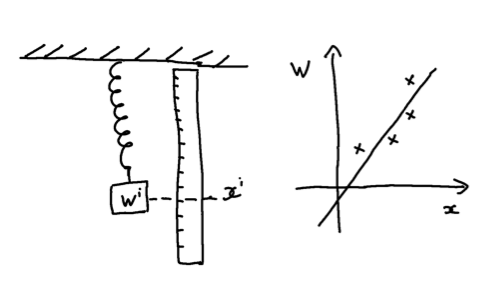
Let’s take Hooke’s law as a concrete example. We are interested in how much a weight attached to a spring stretches it. Usually the relationship is stated with the weight being the independent variable, so we ask, how much weight can the spring support if we stretch it by some amount? In general we can write $W = f(x)$, where $W$ is the weight, and $x$ is the position of that weight. How do we figure out this relationship? We need to start by collecting data, i.e. make an experiment. We make a spring, clamp one end, and the other end hang vertically. Next, we get a set of weights, and start attaching them to the hanging end of the spring. With every added weight the spring is stretched by a certain amount which we can record by attaching a ruler next to the spring.

Now we make a plot of the $W$ against $x$. We find that the plot looks linear, that is we can (almost) connect all of our data points using a straight line. We make the assumption that \(W = \theta_0 + \theta_1 x,\) and try to find the best $\theta_0$ and $\theta_1$ so that we best fit our measurements.

How do we best fit the data? One way is to graphically fit a line by eye. On a physical piece of paper, plot the data, and then with a ruler and pen draw a line such that there is roughly equal number of data points above and below the line. This may be the simplest form of linear regression, and if you have done this exercise in high-school, you have implemented linear regression already.

You might be thinking, if the points are linear, can’t we connect two points by a straight line and then we should have all other points automatically fall onto that line? The reason this doesn’t work is that even in this simple example the data is noisy. There are some unavoidable errors associated with our measurements. For one, we are limited by the accuracy of the ruler, for example. Also the data is collected by a human, and maybe measurements were affected by the parallax effect. Might be that half-way throughout the experiment someone knocked the ruler out of place, and despite your best efforts to put it in the same exact location it wasn’t at exactly the same location. There might also be errors associated with the value of the weights. Maybe one of the weights got a little chip, and we are also limited by the accuracy of the machining process that made the weights. Point being, there are many sources of errors when collecting data in the real world. The errors move the points away from the supposedly true straight line in random directions. Thus connecting two points of data is not a good strategy to obtaining the best-fit line.

My guess is that even high-schoolers don’t do linear fitting by hand anymore. Excel would give you the line of best fit if you feed it the data in no time. How does it figure out the best $\theta_0$ and $\theta_1$? To solve a problem on a computer, we need to write an algorithm. As is usually the case, we can’t formulate the eyeballing method to the computer. Instead, we define a function that describes how far the prediction of our model is from the true data, and then minimize One function that achieves this goal is

where $W^i$ and $x^i$ are the measured weights and positions respectively and $N$ is the number of total measurements made. The further away the prediction of our model, $\theta_0+ \theta_1 x^i$, is from the observed data the larger the loss function. This loss function is called the mean-squared error (MSE). Our job is to find the parameters that give us the smallest possible loss. Formally this is written as

which reads that the optimal $\boldsymbol \theta = (\theta_0, \theta_1)$ are obtained by finding the arguments of the function $\mathcal L(\boldsymbol \theta)$ that minimize it. We will get to how to find these optimal parameters later on.

Linear regression can be used in many contexts. In our spring example, we only had one “feature” that affected the weight attached to the spring, which is the position of the weight. However, in general we might want to consider more than one feature that can have an effect on the output of the model. The canonical example, which I believe was popularized by Andrew Ng (see lecture notes) is predicting housing prices. There are multiple factors that go into how much a house cost, like area, number of rooms, location, when it was built, etc.

In general, the linear model takes the following form x

where $x_\alpha$ and $\theta_\alpha$ are the features and parameters of the model respectively. I will use bold symbols to indicate vectors in the feature space, for example $\boldsymbol x = [x_0, x_1, \dots ]$. Here the convention is that $x_0 = 1$ allowing for a constant term, i.e. the prediction of the model when all features are zero.

Here we encounter the first example showing how tricky understanding a model can be. What is the meaning of $\theta_0$ in the example of predicting house pricing? The price of a house with zero area, number of rooms, … You can already see how silly that sounds. While it is true that this is what the model would spit out when we input a data point with $x_\alpha = 0, \forall \ \alpha> 0$, saying that the meaning of $\theta_0$ is the price of a house with these features is a meaningless statement. There is no such house. I wanted to point this out. I’ll leave discussion about interpretability for another blog.

Linear regression model as a statistical model

Let’s get back to the loss function. Why not take absolute values, or powers of $4$ of the errors? One can derive the MSE loss function by looking at the linear regression model as a statistical model. We already mentioned how errors are unavoidable when collecting data. Thus in general we should expect

where $\epsilon$ quantifies the errors we make. To know what is $\epsilon$, we need to have a model for the errors. The most natural, and common choice is to take the errors to follow a gaussian distribution. So rather than saying that given the features $x_\alpha$ our prediction is certainly $y_{\boldsymbol \theta}(\boldsymbol x)$, we have a probability distribution. We ask, given the features $x_\alpha$ what is the probability that we make a prediction $y$? This is written as $p(y|\boldsymbol x)$, and in the case of the normal distribution is given by

Our linear model makes predictions about the mean of the normal distribution

In other words, the model makes predictions by giving its best guess of what the mean of the distribution is. The data set is a list of $(y^i, \boldsymbol x^i)$, where $y^i$ is the effect we are trying to model, and $\boldsymbol x^i$ are the features that determine that effect. We denote the list of all $y^i$’s as $Y = [y^0, y^1 , \dots, y^{N-1} ]$ and the list of all $x^i$’s as $\boldsymbol X = [\boldsymbol x^0, \boldsymbol x^1, \dots, \boldsymbol x^{N-1}]$. In our notation, a bold symbol is a vector in the feature space, and a capital letter symbol is a list of the data. A bold capital letter means it is the data list of the features vectors. We can think of $\boldsymbol X$ as a matrix, the components of which are given by $\boldsymbol X_{i \alpha} = x^i_\alpha$.

The probability of $Y$ given $X$ is the product of all $p(y^i|\boldsymbol x^i;\boldsymbol \theta)$

When we view $p(Y|X; \boldsymbol \theta)$ as a function of the parameters $\boldsymbol \theta$, we call this function the likelihood of the parameters

I won’t get too much into a discussion of probability vs. likelihood. Maybe in another blog.

The best model parameters are those that maximize the likelihood $L(\boldsymbol \theta)$. We find the maximum likelihood by minimizing minus its log. The reason this works is because the log is a monotonic function. The reason this is a good idea is that it gives a simple expression to work with

We thus see that 1. Minimizing minus log of the likelihood is the same as maximizing the likelihood of the parameters, and that 2. Minimizing the minus log of the likelihood is the same as minimizing the MSE between $y^i$ and the mean of the normal distribution, which is the model prediction.

Where does the name regression come from?

This part is probably not important and you can skip if you want. However, the name regression always sounded weird to me. Why not call it linear fitting? According to the Wikipedia page on regression analysis, the name comes from the statistical phenomena of “regression to the mean”. Veritasium has a nice video explaining this concept. I’ll summarize here with a silly example. Suppose you roll a $1000$ dice. The mean of the numbers on the faces would be close to $3.5$. If we take the dice with faces showing $5$ and $6$ which have an average of about $5.5$ and roll them again, then the mean of these dice would regress back from $5.5$ to something much closer to mean of the original distribution which is $3.5$. Basically there is nothing inherently special about the dice that was showing high numbers on the first run, and if we roll them again they perform like all other dice. The same effect can show up in more subtle situations. I’ll refer to the Veritasium video for an interesting example.

As we alluded to already, when collecting our data, we are sampling from some probability distribution (because of the errors associated with measurements), the mean of which have a linear relationship with the model features. So are we predicting the mean the data is regressing to? I am not convinced this is a good name, but okay. Let me know if you have a better explanation.

Normal equation for the parameters

A nice feature of the linear model is that there is a closed form for the optimal parameters. In matrix form, the loss function takes the following form

To find the minimum of $\mathcal L(\boldsymbol \theta)$ we need to set the derivatives with respect to all parameters to zero $\partial \mathcal L (\boldsymbol \theta) / \partial \theta_\alpha = 0\ \forall \ \alpha$. For ease of notation, we define

When taking the derivative of $(1)$, with respect to $\theta$ the first term doesn’t depend on $\theta$, the second and third terms are equal, and so are the derivatives

The derivative of the quadratic term (the last term) in Eq. (1) is somewhat less obvious, at least for me. The way I remind myself of how to do it is by adding a small term to the variable we are taking the derivative for and collect the linear terms

collecting the first order terms in $\delta \boldsymbol \theta$ we find that the change we make is

and thus in the limit of $\delta \boldsymbol \theta \rightarrow 0 $

Putting everything together we have

Setting the derivative to zero we get an equation for the optimal parameters

There might be some subtleties with inverting the matrix $\boldsymbol X^T \boldsymbol X $, but that is outside the scope of this blog for now. I just wanted to highlight that there exists a closed form solution.

Limitations of the linear model

It comes as no surprise that a lot of our world is not linear, making the limitations of the linear model pretty obvious. However, one can easily expand its scope by feature engineering. Suppose you want to build a linear model to predict the range an electric car has on a single charge. To make things simple, let’s assume highway driving, so no stopping and starting. You know that the range should depend on the speed you are driving with. You might build the model for the range with a linear term $\beta_v v$ where $v$ is the speed you are driving with. A negative $\beta_v$ would indeed give us the correct behavior of decreasing range with increasing velocity. However such model is not accurate, since the relationship between the range and velocity is inherently non-linear. If we have a bit of knowledge about drag forces we might add the following term to the model $\tilde \beta_v \frac{1}{v^2}$. Such term should improve the accuracy of the model since it includes the correct scaling of drag forces with velocity. Including this term in the model is what is known as feature engineering. In this example, we had a good idea of what is the correct feature to include. In more complex situations we might not know. Going back to the housing pricing example, we might expect that at some point, the bigger the areas of a house the price would shoot upwards not in a linear fashion, maybe because we are now in a different category of real-estate, like moving from the realms of apartments to houses or form houses to mansions.

Another limitation of the linear model is that it ignore correlation between features. In the housing prices example, we should expect location and area to be correlated. A slightly bigger house in a desirable location might cost a lot more than a slightly bigger house in a less desirable location, for example. A model with terms $\theta_{\text{area} } (\text{area} ) + \theta_{\text{location} } (\text{location} ) $ can never capture this effect.

One can add an interaction terms to the linear model to capture such effects. For example we can add $\theta_{\text{int}} (\text{area}) (\text{location})$. The obvious limitation is that we are not sure what is the correct form of the interaction and we can only guess in many situations. The other drawback is now terms in the model are not independent, and this makes understanding the model a lot more opaque. What is the meaning of the $\theta_{\text{area}}$ when we also have $\theta_{\text{int}}$? How much the price would change if we changed the area with other features being equal is suddenly a meaningless statement.

Linear models are very capable for what they are. They are easy to implement, and they seem to perform well in many cases. If we can also limit the model to small number of features, then their predictions are easy to understand by a human. All these factors make them very popular and appealing to use. They are probably a good starting point if we are tackling a problem we don’t have much experience with.

In this blog:

1. I describe how the simple OLA I trained previously is nothing but a linear regression model.
2. Show how to modify the training as to allow OLA to be non-linear
3. Show that for the task of predicting dynamics with fixed natural frequency and damping, the model learns to reduce to a linear model.
4. Study the model behaviour for the harder task of training the model with variable natural frequency and damping.
5. Study whether the model reduces to a linear model in the variable-parameter setting.

Let’s start with a quick recap of the last blog post. The dynamics of the harmonic oscillator can be described using the following linear equation

where $x(t)$ is the position, and $p(t)$ is the momentum and $K(\omega_0, \gamma, \Delta t)$ is a $ 2 \times 2$ matrix that carries all the information about the dynamics of the harmonic oscillator with frequency $\omega_0$ and damping $\gamma$.

I train an OLA model to try to learn this dynamics. Formally, the OLA applies the following series of transformations

with

Here the input $\boldsymbol X = [ (x_1,p_1), (x_2,p_2), \ldots, (x_T,p_T)]$ is $n$ time steps of the dynamics, and the output $Y = (x^{\text{pred}}_{T+1}, p^{\text{pred}}_{T+1})$ is what we hope to make as close as possible to the true $(x_{T+1}, p_{T+1})$. We used the following MSE loss function in training

Please refer to the last blog post for more detail.

There is such a thing as too simple

I wanted to start simple. So I fixed $\omega_0$ and $\gamma$. In this case, the model does not need to attend beyond the $t$-th time step to predict the $t+1$ time step. Thus I restricted the attention to just one time step back. However, what I didn’t fully realize is that in doing so I basically reduced the model to a linear model. This is embarrassingly easy to see. If the attention matrices $A^\alpha$ are fixed, then the model is linear. The only non-linearity in the model comes from the softmax in the attention

Now, if we restrict $A$ to only attend to one time step back this fixes the attention matrix, and the result of the softmax function is $1$ for the $t$-th time step and zero otherwise regardless of the value of $\boldsymbol X$. So, I managed to reduce the model too much, as indeed given the linear nature of the problem, one could just as well have trained a linear regression model and it would have been just as successful.

As I mentioned before, my intentions are not to train a model to do something ground breaking, but to see how transformers can do physics. But here I managed to simplify too much as to remove the character of the attention mechanism. Silly me.

The obvious thing to do is to allow the model to attend to multiple time steps back. This is an overkill for our problem, but do we gain any insight into the inner workings of attention by doing so? Before we look at the performance of the OLA model in this setup, let’s compare with a linear model to predict the next time step:

where $X_{t} = (x_t, p_t)$ with the convention that $X_{0} = [1, 1]$ to add a constant term to the sum, and $\beta_t \in \mathbb R^{2\times 2}$. What is the difference between this model and the attention model? Can’t we think of $\beta_t$ as some sort of attention? The difference is that for the linear model, the structure is rigid, and independent of the input of the model. Attention is input dependent such that the OLA model can attend to different time steps for different inputs. I guess this is in part what makes attention powerful in natural language processing setting, where depending on the sentence, the model needs to attend to different parts.

Saliency map

Now, does the OLA model do anything interesting when allowed to attend to multiple time steps back? Before we get to this question, I want to mention a change of the loss function that I had to make for the model to train successfully. First, we change the output of the model for a given input $ \boldsymbol X = [ (x_1,p_1), (x_2,p_2), \dots \ (x_T,p_T)]$ to be $\boldsymbol{Y} = [(x^\text{pred}_2,p^\text{pred}_2), (x^\text{pred}_3,p^\text{pred}_3), \dots \ (x^\text{pred}_{T+1},p^\text{pred}_{T+1})] $, and define the loss function to be

This loss function is more in line with how transformers are usually trained as I understand. As to why this loss function works better than the one in Eq. (1) I can’t say I fully understand. Though I suspect it has something to do with how gradients scale with $T$, as how they flow through the network. Maybe I’ll explore this later.

Using $T = 40$ with a causal mask on the attention matrix, the model trains well as shown in Fig. 1.

Fig. 1: OLA model training results with $T = 40$ time steps.

Does the model do anything with all the new bandwidth given? This does not seem to be the case. The model here learns to reduce itself to a linear model, eliminating the attention module altogether. This can be first seen by looking at the saliency map. A saliency map in its simplest form tells you how the outputs of the model are changed as you change the inputs. In our notation the output is $\boldsymbol Y_t = (x^{\text{pred}}_{t+1}, p^{\text{pred}}_{t+1})$ and $\boldsymbol X_t = (x_t, p_t)$, and the saliency plot is a map of $\partial Y^\alpha_i / \partial X^\beta_j$ as shown in Fig. 2.

Fig. 2: Saliency map for OLA model with $T = 40$.

The fact that the saliency map is diagonal means that the values of previous tokens do not affect each other. One can further confirm this by looking at the output matrix $W_O$ and in this case we see that it has zeros for all elements. That is, the attention actually writes nothing to the residual stream…

Admittedly this is a whole lot of work for nothing.

Except it is not really for nothing. We learned something. We want to see the attention mechanism in action in the simplest case possible, and our approach here is to start as simple as we can and only make things more complex when we are forced to. We also got familiar with transformers and set the notations.

Making things as complex as they need to be

We need to make the problem harder such that it is no longer linear. I think the simplest, and most interesting way to do this is to allow the natural frequency and damping to vary during training. This forces the model to first learn $\omega_0$ and $\gamma$ from the given input path, then make the prediction for the next time step.

For now, I keep $\gamma$ fixed, and train the model with trajectories having $\omega_0 \in [1.0,4.0]$ and $\gamma = 0.1$. This is how the model performs when given a trajectory with $\omega_0 = 2.0$ at validation

Fig. 3: OLA model cannot learn $\omega_0$ when trained on trajectories with different $\omega_0$.

The model fails to reproduce the dynamics except for a very small number of time steps, and then quickly becomes very wrong. There are many ways we can try to increase the complexity of the model to try to enhance its performance. First thing to try is to increase the dimensions of the residual stream. Here are the results with $d_{\text{model}} = 8$, and $d_{\text{head}} = 4$:

Fig. 4: Changing the residual stream dimensions as well as using 2 attention heads does not seem to help.

This seems to perform worse and does not help.

Next we try moving to a more complicated model. Instead of the one layer attention, we try n-layer attention model (nLA). Here are the results for $n = 8$ with $d_{\text{model}} = 16$, and $d_{\text{head}} = 8$:

Fig. 5: Adding more attention layers doesn’t seem to help either

This doesn’t seem to do much of anything either.

Interestingly, what seems to help a lot is removing the causal mask in the attention mechanism:

Fig. 6: Removing the causal mask from the attention mechanism seems to help with training and performance quite a bit

I initially added the causal mask because it seemed like a nice physical constraint. However, I don’t see any reason that you must have it. There is no cheating here by removing the causal mask. Increasing the number of layers in the case of no causal attention helps model prediction:

Fig. 7: Adding more layers when we remove causal mask helps performance.

Finally, a quick comparison with linear models. Two things I want to address: 1. How does the performance of the $n$-LA model compare to a simple linear model, and 2. Does the $n$-LA model reduce to a linear model similar to before. I think the following plot addresses both questions:

Fig. 8: Comparing $n$-LA model with a linear regression model. Also using a linear model as a surrogate model to see if the $n$-LA model reduces to a linear model.

In the above plot, the model is the $n$-LA model with $n = 8$. At least to my eye, the $n$-LA model seems to track the true trajectory better. Furthermore, we train a surrogate linear model for the $n$-LA model. If the $n$-LA model got reduced to something that is linear then we should be able to train a surrogate model to exactly reproduce its behaviour. This does not seem to be the case, as the trajectory of the surrogate model quickly diverges from that of the original model. I take that as strong evidence that the $n$-LA is not reduced to a linear model.

I’ll have to keep experimenting with the transformer model to improve its accuracy. If you see a reason this task is doomed to fail let me know. If you have ideas about how to make the model better also let me know.

These blog posts are my notes, and progress updates. I am curious how far I can get with this. Hopefully posting small progress updates can keep me motivated.

My strategy to make progress is the following:

1. Train a transformer model to solve a simple physics problem that is very well understood.
2. Develop tools to probe how the model solves the problem.

Step 1 is easier than step 2 in that it is a well defined problem with a lot of work and knowledge already developed to address it. Step 2 is the real challenge. We’ll get to that in due time.

The problem I picked for step 1 is the classical simple harmonic oscillator: a mass $m$ attached to a spring with a spring constant $k$ and damping $\gamma$. The equation of motion is $\ddot x + 2\gamma \dot x + \omega_0^2 x = 0$. Here I’ll focus on the underdamped case $\omega > \gamma$. We take $m = 1$ throughout.

The model

My motive in designing the model is to pick the simplest transformer model that can do the task, so that when time comes for interpreting the model we would have an easier task. The simplest transformer model is the single layer attention only transformer. Here we describe this model, and how it does predictions.

Whatever model we define is tasked with the following: given a sequence of points in the phase space $\boldsymbol X = \{(x_0,p_0), (x_1,p_1), \dots \ (x_n,p_n)\}$ representing the dynamics of the system $(x_i,p_i) = (x(n\Delta t), p(n\Delta t))$, where $\Delta t$ is some small time step, what is the next point in the time series $\boldsymbol Y = (x_{n+1} , p_{n+1})$. A model that does this well, can also generate full trajectories by appending $\boldsymbol Y$ to $\boldsymbol X$ and feed this back to the model to generate $(x_{n+2}, p_{n+2})$ and so on.

The simplest transformer model is the single layer, attention-only transformer. For the following we think of $\boldsymbol X \in \mathbb R^{2\times n}$ as a matrix with rows representing position and momentum, and columns representing the time index. The transformer model then does the following computations,

where $W_E$, and the $W_U$ are the embedding and unembedding matrices respectively. $W_E$ maps the input to the model residual stream of dimension $d_{\text{model}}$, and $W_U$ maps back to position and momentum at the end of the computation. Thus, $\tilde{\boldsymbol X} \in \mathbb R^{d_{\text{model}} \times n}$ and $\tilde{Y} \in \mathbb R^{d_{\text{model}} \times 1}$. Finally we have the prediction $\boldsymbol Y \in \mathbb R^{2\times 1}$. The model we train has $d_{\text{model}} = 2$ in the spirit of keeping things as simple as they can be.

Here $h(\tilde{\boldsymbol X})$ is the attention later action on the residual stream. We quickly review what it does. Though by now, the Internet is filled with resources that can teach you about this in much more detail. Each attention layer (for which we only have one) consists of multiple attention heads $n_{\text{head}}$. Each head act on a subspace $d_{\text{head}}$ of the residual stream (of dimension $d_{\text{model}}$). Usually one asserts that $d_{\text{model}} = n_{\text{head}} d_{\text{head}}$. The result of the attention layer is the sum of the action of each attention head

There are two parts to each attention head: 1. The value-output part, which determine what to read from the residual stream and which subspace to write into. 2. The key-query part which determine what “tokens”, in our case which time steps, to attend to, and by how much. Together the action takes this form

\(h^\alpha(\tilde{\boldsymbol X}) = W^\alpha_O W^\alpha_{V} \tilde{\boldsymbol X} A^\alpha\) where $A$ is the attention matrix defined as

A causal mask is applied to the attention matrix such that the model can only attend to previous time steps.

The model is thus defined by the weights of the six matrices $W_E, W_U, W_Q, W_K, W_V, W_O$ and optionally also two biases $b_E$ and $b_U$ added to the embedding and unembedding layers. A very important parameter of the model is how many time steps back (tokens) do we allow the model to look at to make prediction. For the simple harmonic oscillator, with fixed natural frequency $\omega_0$ and damping $\gamma$ the model in principle only need to see $(x_n, p_n)$ to make the prediction about $(x_{n+1}, p_{n+1})$. With this in mind we only train model attending only to the previous time step.

Data generation and training

Here we describe how we generate the training data. That is, how to go from $(x_n, p_n)$ to $(x_{n+1}, p_{n+1})$ for any $\Delta t$. The damped harmonic oscillator has an analytical solution. For the underdamped case we have the general solution

where $\omega = \sqrt{\omega_0^2 + \gamma^2}$. This allows us to write the following update rule for $x$ and $p$ for an arbitrary time step $\Delta t$,

This is everything to need to start training the model.

The model is trained to make a single forward time step prediction. We generate multiple $(x^i_0, p^i_0)$ starting points. The model makes predictions $(x^i_1, p^i_1)$. The true values $(\hat x^i_1, \hat p^i_1)$ are generated as described above. We use a mean square error as the loss function to be minimized

where $N$ is the number of samples generated.

We use AdamW as an optimizer, and use batches of the generated sample at each step of the optimization process.

Results

How well does the model perform? For training with fixed $\omega$ and $\gamma$ the model trains very well. We train the model using points $(x_0, p_0)$ with energies $E = \frac{1}{2} (p^2 + \omega^2 x^2)$ in a range $[0, E^{\text{train}}_{\text{max}}]$. We perform validation for trajectories with energies in the range $[0, E^{\text{valid}}_{\text{max}}]$ with $E^{\text{valid}}_{\text{max}} > E^{\text{train}}_{\text{max}}$ to test if the model generalizes to trajectories not seen in training. We also roll out the full trajectory. We start by inputting $(x_0, p_0)$, make a prediction $(x^{\text{pred}}_1, p^{\text{pred}}_1)$, then feed $(x^{\text{pred}}_1, p^{\text{pred}}_1)$ back to the model to get $(x^{\text{pred}}_2, p^{\text{pred}}_2)$ and so on.

Here is an example of the results for $\gamma = 0$:

And here is an example with damping included $\gamma \neq 0$,

First, even after $200$ steps, the relative errors in both cases are very small $~10^{-4}$. What is impressive also is that the error does not seem to be getting bigger with time. There is the spikes here and there, but on average the model is performing great on the full trajectory despite being only trained on just next step prediction.

What is next

I think even at this step there is are interpretability questions to be asked, and if answered properly can be useful in understanding bigger models. It seems that the model learns the natural frequency and the damping of the harmonic oscillator. I think the following two questions need to be addressed:

1. Can we confirm that the model indeed learned $\omega_0$ and $\gamma$? Ideally we want to confirm this by asking questions about the attention layer.
2. If we can conform that the model learned $\omega_0$ and $\gamma$, how does the model make predictions? Does it use something similar to the update rule we defined above, or did it come up with some other way?

What does it mean for a machine learning (ML) model to have learned a “concept” related to the task it’s doing? This is a hard question to answer because a “concept” is one of these things we have no issue using in our everyday language, but when you sit down and actually try to properly define, it is hard to pin down. This blog will discuss this issue, and why it might be important for discovering new science.

Most of us now interact with ML models through chat bots. At least in the early days of starting using these bots, the first question people tend to ask is whether they actually understand the conversation. It is very hard to gauge “understanding”, even in real humans, speaking from experience of years trying to teach students about physics. People much smarter than me have tried to give an appropriate definition. I’ll give one of my own later on. Historically, it seems that saying a network has learned a concept is a you “know it when you see it” kind of thing. An example is the best way to explain this. This example is from the world of natural language processing. Consider a network that takes as an input an $N$-gram (a sequence of $N$ words that make a sentence or are part of a sentence). The output of the network is to determine whether this $N$-gram is proper English. For example “the dogs are playing outside” is a valid $5$-gram, whereas “the chairs are playing outside” is not a valid $5$-gram (at least not in our world). One can construct the training data quite easily. Start with any corpus, take every $N$-grams and label them as the valid grams. From a valid $N$-gram, if we randomly substituted a single word, it’s very likely that we end up with an $N$-gram that is invalid.

The neural network will have multiple layers to be able to perform the task of determining whether an $N$-gram is valid English or not. For our example, we only need to focus on the representation layer. The job of the representation layer is to take every word $x$ and map it to to a vector in a, let’s say, $50$-dimensional space $w(x)$. The way words are represented using $w(x)$ is not something that we impose on the network. Instead, we let this representation be part of what the network learns during training. The hope is that the learned representation carry information about relationships between different work that would aid the network performing its ultimate goal.

After training is done, the network learns to cluster words of similar meaning close to each other. For example one would find $||w(\text{dog}) - w(\text{dogs})|| \ll ||w(\text{dogs}) - w(\text{cats})|| \ll ||w(\text{dog}) - w(\text{chair})||$. What is more fascinating, and what really started my interest about subject, is that the network seems to learn semantic relationships between words as well! For example, if we look at the vectors $c_1 = w(\text{king}) - w(\text{queen})$ and $c_2 = w(\text{uncle}) - w(\text{aunt})$, we find that $c_1 \approx c_2$. One might form the hypothesis that $c_1 \approx c_2 \approx c_{\text{gender}}$, i.e. the vector that carry the concept of gender.

I want to take a second here to emphasis what qualifies as a hypothesis, from the point of view of doing science. For a statement to qualify as hypothesis it need to be falsifiable. If we cannot come up with a test, were one of the outcomes would disprove the hypothesis, then it is no good. This is the foundation for doing science. Fortunately, we can come up with a test for our $c_{\text{gender}}$ hypothesis. We can predict the position for the embedding of the word, let’s say, “father”, using $w(\text{father}) = w(\text{mother}) + c_{\text{gender}}$. Of course what we really need to do is look for the word with the closest vector to $w(\text{mother}) + c_{\text{gender}}$, but I’ll gloss over such detail. Indeed, with a good degree of accuracy the hypothesis hold. As you can probably already imagine, we can construct similar vectors for other concepts as well.

I think most people would agree that in the above example, the network has learned concepts in a way that we can understand. There are other instances where ML models have shown that it can behave, based on its training, in a way that is much less understood by humans. Take the example of AlphaGo’s game against Lee Sedol who’s regarded to be the best Go player (though don’t quote me on that, I’m sure some people might disagree). On move 37 of one of the games AlphaGo made a very unusual move that confounded all commentators, spectators, and Lee Sedol himself. AlphaGo would win that game, and move 37 would become very popular (as featured in the documentary by DeepMind) as a move where AlphaGo demonstrated knowledge, and understanding of the game that is beyond human knowledge and understanding. This is certainly such an interesting prospect. Can we train models such that they would learn something we never learned before? This certainly seems plausible, but immediately begs the question: how do we extract this knowledge? Unbeknownst to me, there is a whole branch of ML/AI research dedicated to this problem of interpretability.

Back to the question in the title. What does this all mean for physics. ML models have been used in various physics applications. Since I’m not familiar with the field, I want to start with something simple.
As Sidney Coleman would say, “The career of a young theoretical physicist consists of treating the harmonic oscillator in ever-increasing levels of abstraction.” I don’t believe I’m considered young anymore, but I also don’t think Coleman had studying the harmonic oscillator using ML in mind either. Anyway, if you are not familiar, a harmonic oscillator is a body with mass $m$ that is attached to a spring with a spring constant $k$. Classically, the one-dimensional harmonic oscillator state is fully described by its position $x$ and momentum $p$. We can try to train an ML model to learn the dynamics of this system. One way to train this model is to give the model $X = (x_0,\ p_0,\ t)$ and ask it to output $Y = (x(t), \ p(t))$. With the help of ChatGPT, I built a neural network with $4$ hidden layers ($16$ units in the first and last layers, and $32$ units in the middle two). Training this network on $5\times 10^4$ samples of $(X,Y)$, yields pretty dismal results to be honest. I was curious, I had to try. Here is a plot for the predicted trajectory of the model:

One can say the model learned something about the system. The trajectory kind of resemble a circle (as it should). But even in this very simple of examples it is very hard to say what exactly has the model learned.

I think to be able to say the model has learned something one should be able to formulate this something as a hypothesis. Remember, the most important pillar of an hypothesis is that it needs to be falsifiable. In the harmonic oscillator example, one might form the hypothesis that the model learned about conservation of energy. Testing this hypothesis is easy. For a set of outputs of the model $(x(t), \ p(t))$ compute the energy $E(t) = p^2(t)/2m + kx^2(t)/2$, and see if it is a function of time. Our neural network above clearly didn’t learn about conservation of energy, and thus the hypothesis is false in this case.

In the literature, there are multiple attempts to try to solve the harmonic oscillator by designing networks that automatically respect energy conservation. This is not really the point of this exercise. We are not trying to teach the network some concept that we humans already know. What I’m interested in here is trying to train the network somewhat agnostically, and see if gradient descent imposed some structure on the network that we can study and learn something new from. Of course in this regard the harmonic oscillator is a bad example since we understand every aspect of it.

Note that defining a concept as a hypothesis about the behavior of the network is rather stringent. For example, move 37, while impressive, cannot be formulated as a hypothesis. In my view, taking such definition of a concept learned by a network is the first step to bring interpretability work more within the realms of science. How else can we deal with fuzzy concepts?

The interesting prospect at the intersection of interpretability and physics is the following: can we reach a point where we train a model that is very good in predicting physical phenomena that our best bet to understand these phenomena is to understand the model we created. I certainly don’t know the answer to this question, but the thought of such possibility makes me excited about this area of research.