Transformer models have been used in the physics literature to solve many interesting problem. While these models have proved their utility as tools, it is not clear how they solve these problems. This blog is the first in a series of blogs that tries to address the question of what transformer models actually learns when trained to solve a physics problem. The goal here is not to train a model to do something impressive, but rather, given a well trained model can we interpret how the model solves the problem. Can we look inside the model and ask if it has learned physics concepts. In my view this is an interesting question because of the prospect of potentially seeing old physics in new light. Maybe we can learn some new perspective from these models. I have discussed this motive in a previous blog post.
These blog posts are my notes, and progress updates. I am curious how far I can get with this. Hopefully posting small progress updates can keep me motivated.
My strategy to make progress is the following:
- Train a transformer model to solve a simple physics problem that is very well understood.
- Develop tools to probe how the model solves the problem.
Step 1 is easier than step 2 in that it is a well defined problem with a lot of work and knowledge already developed to address it. Step 2 is the real challenge. We’ll get to that in due time.
The problem I picked for step 1 is the classical simple harmonic oscillator: a mass $m$ attached to a spring with a spring constant $k$ and damping $\gamma$. The equation of motion is $\ddot x + 2\gamma \dot x + \omega_0^2 x = 0$. Here I’ll focus on the underdamped case $\omega > \gamma$. We take $m = 1$ throughout.
The model
My motive in designing the model is to pick the simplest transformer model that can do the task, so that when time comes for interpreting the model we would have an easier task. The simplest transformer model is the single layer attention only transformer. Here we describe this model, and how it does predictions.
Whatever model we define is tasked with the following: given a sequence of points in the phase space $\boldsymbol X = \{(x_0,p_0), (x_1,p_1), \dots \ (x_n,p_n)\}$ representing the dynamics of the system $(x_i,p_i) = (x(n\Delta t), p(n\Delta t))$, where $\Delta t$ is some small time step, what is the next point in the time series $\boldsymbol Y = (x_{n+1} , p_{n+1})$. A model that does this well, can also generate full trajectories by appending $\boldsymbol Y$ to $\boldsymbol X$ and feed this back to the model to generate $(x_{n+2}, p_{n+2})$ and so on.
The simplest transformer model is the single layer, attention-only transformer. For the following we think of $\boldsymbol X \in \mathbb R^{2\times n}$ as a matrix with rows representing position and momentum, and columns representing the time index. The transformer model then does the following computations,
\[\begin{align} \boldsymbol X &\rightarrow \tilde{\boldsymbol X} = W_E \boldsymbol X \nonumber \\ \tilde{\boldsymbol X} &\rightarrow \tilde{\boldsymbol Y} = \tilde{\boldsymbol X} + h(\tilde{\boldsymbol X}) \nonumber \\ \tilde{\boldsymbol Y} &\rightarrow \boldsymbol Y = W_{U} \tilde{\boldsymbol Y} \nonumber \end{align}\]where $W_E$, and the $W_U$ are the embedding and unembedding matrices respectively. $W_E$ maps the input to the model residual stream of dimension $d_{\text{model}}$, and $W_U$ maps back to position and momentum at the end of the computation. Thus, $\tilde{\boldsymbol X} \in \mathbb R^{d_{\text{model}} \times n}$ and $\tilde{Y} \in \mathbb R^{d_{\text{model}} \times 1}$. Finally we have the prediction $\boldsymbol Y \in \mathbb R^{2\times 1}$. The model we train has $d_{\text{model}} = 2$ in the spirit of keeping things as simple as they can be.
Here $h(\tilde{\boldsymbol X})$ is the attention later action on the residual stream. We quickly review what it does. Though by now, the Internet is filled with resources that can teach you about this in much more detail. Each attention layer (for which we only have one) consists of multiple attention heads $n_{\text{head}}$. Each head act on a subspace $d_{\text{head}}$ of the residual stream (of dimension $d_{\text{model}}$). Usually one asserts that $d_{\text{model}} = n_{\text{head}} d_{\text{head}}$. The result of the attention layer is the sum of the action of each attention head
\[h(\tilde{\boldsymbol X}) = \sum_{\alpha \in \\{1, \dots n_{\text{head}}\\} } h^\alpha (\tilde{\boldsymbol X}).\]There are two parts to each attention head: 1. The value-output part, which determine what to read from the residual stream and which subspace to write into. 2. The key-query part which determine what “tokens”, in our case which time steps, to attend to, and by how much. Together the action takes this form
\(h^\alpha(\tilde{\boldsymbol X}) = W^\alpha_O W^\alpha_{V} \tilde{\boldsymbol X} A^\alpha\) where $A$ is the attention matrix defined as
\[A^{\alpha}_{ij} = \text{Softmax}\left( \frac{[\tilde{\boldsymbol X}^T W_K^T W_Q \tilde{\boldsymbol X]_{ij}}}{\sqrt{d_{\text{model}}}} \right) = \frac{\exp\left[{\frac{[\tilde{\boldsymbol X}^T W_K^T W_Q \tilde{\boldsymbol X]_{ij}} }{\sqrt{d_{\text{model}}}}} \right ] }{\sum_{i} \exp\left[\frac{[\tilde{\boldsymbol X}^T W_K^T W_Q \tilde{\boldsymbol X]_{ij}}}{\sqrt{d_{\text{model}}}}\right] }.\]A causal mask is applied to the attention matrix such that the model can only attend to previous time steps.
The model is thus defined by the weights of the six matrices $W_E, W_U, W_Q, W_K, W_V, W_O$ and optionally also two biases $b_E$ and $b_U$ added to the embedding and unembedding layers. A very important parameter of the model is how many time steps back (tokens) do we allow the model to look at to make prediction. For the simple harmonic oscillator, with fixed natural frequency $\omega_0$ and damping $\gamma$ the model in principle only need to see $(x_n, p_n)$ to make the prediction about $(x_{n+1}, p_{n+1})$. With this in mind we only train model attending only to the previous time step.
Data generation and training
Here we describe how we generate the training data. That is, how to go from $(x_n, p_n)$ to $(x_{n+1}, p_{n+1})$ for any $\Delta t$. The damped harmonic oscillator has an analytical solution. For the underdamped case we have the general solution
\[x(t) = \text{Re} \ A e^{-(\gamma + i \omega)t}\]where $\omega = \sqrt{\omega_0^2 + \gamma^2}$. This allows us to write the following update rule for $x$ and $p$ for an arbitrary time step $\Delta t$,
\[\begin{bmatrix} x(t + \Delta t) \\ p(t + \Delta t) \end{bmatrix} = e^{-\gamma \Delta t} \begin{bmatrix} \cos(\omega \Delta t ) + \frac{\gamma}{\omega} \sin(\omega \Delta t ) & \frac{1}{\omega} \sin(\omega \Delta t ) \\ \frac{-\omega^2_0 }{\omega} \sin(\omega \Delta t ) & \cos(\omega \Delta t ) - \frac{\gamma}{\omega} \sin(\omega \Delta t ) \end{bmatrix} \begin{bmatrix} x(t) \\ p(t) \end{bmatrix}\]This is everything to need to start training the model.
The model is trained to make a single forward time step prediction. We generate multiple $(x^i_0, p^i_0)$ starting points. The model makes predictions $(x^i_1, p^i_1)$. The true values $(\hat x^i_1, \hat p^i_1)$ are generated as described above. We use a mean square error as the loss function to be minimized
\[MSE = \frac{1}{N} \sum_i [(x^i_1 - \hat x^i_1)^2 + (p^i_1 - \hat p^i_1)^2]\]where $N$ is the number of samples generated.
We use AdamW as an optimizer, and use batches of the generated sample at each step of the optimization process.
Results
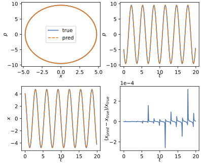
How well does the model perform? For training with fixed $\omega$ and $\gamma$ the model trains very well. We train the model using points $(x_0, p_0)$ with energies $E = \frac{1}{2} (p^2 + \omega^2 x^2)$ in a range $[0, E^{\text{train}}_{\text{max}}]$. We perform validation for trajectories with energies in the range $[0, E^{\text{valid}}_{\text{max}}]$ with $E^{\text{valid}}_{\text{max}} > E^{\text{train}}_{\text{max}}$ to test if the model generalizes to trajectories not seen in training. We also roll out the full trajectory. We start by inputting $(x_0, p_0)$, make a prediction $(x^{\text{pred}}_1, p^{\text{pred}}_1)$, then feed $(x^{\text{pred}}_1, p^{\text{pred}}_1)$ back to the model to get $(x^{\text{pred}}_2, p^{\text{pred}}_2)$ and so on.
Here is an example of the results for $\gamma = 0$:
And here is an example with damping included $\gamma \neq 0$,
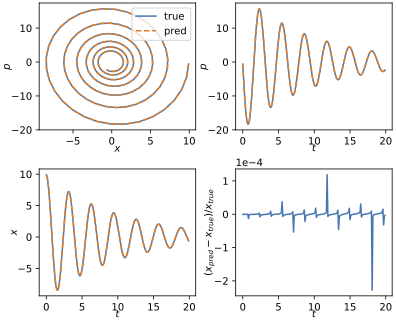
First, even after $200$ steps, the relative errors in both cases are very small $~10^{-4}$. What is impressive also is that the error does not seem to be getting bigger with time. There is the spikes here and there, but on average the model is performing great on the full trajectory despite being only trained on just next step prediction.
What is next
I think even at this step there is are interpretability questions to be asked, and if answered properly can be useful in understanding bigger models. It seems that the model learns the natural frequency and the damping of the harmonic oscillator. I think the following two questions need to be addressed:
- Can we confirm that the model indeed learned $\omega_0$ and $\gamma$? Ideally we want to confirm this by asking questions about the attention layer.
- If we can conform that the model learned $\omega_0$ and $\gamma$, how does the model make predictions? Does it use something similar to the update rule we defined above, or did it come up with some other way?