In my previous blog post I discussed training a one-layer attention-only model to solve the harmonic oscillator. I am going to refer to this model as the one layer attention (OLA) model. My motivation for training this model is to see if transformers can solve the problem in a novel way. The model was successful, but as it turned out I made the model too simple as to basically reduce it to a linear model. Quite embarrassing in retrospect. However, I feel like I learned something in the process, and I hope you do too.

In this blog:

1. I describe how the simple OLA I trained previously is nothing but a linear regression model.
2. Show how to modify the training as to allow OLA to be non-linear
3. Show that for the task of predicting dynamics with fixed natural frequency and damping, the model learns to reduce to a linear model.
4. Study the model behaviour for the harder task of training the model with variable natural frequency and damping.
5. Study whether the model reduces to a linear model in the variable-parameter setting.

Let’s start with a quick recap of the last blog post. The dynamics of the harmonic oscillator can be described using the following linear equation

where $x(t)$ is the position, and $p(t)$ is the momentum and $K(\omega_0, \gamma, \Delta t)$ is a $ 2 \times 2$ matrix that carries all the information about the dynamics of the harmonic oscillator with frequency $\omega_0$ and damping $\gamma$.

I train an OLA model to try to learn this dynamics. Formally, the OLA applies the following series of transformations

with

Here the input $\boldsymbol X = [ (x_1,p_1), (x_2,p_2), \ldots, (x_T,p_T)]$ is $n$ time steps of the dynamics, and the output $Y = (x^{\text{pred}}_{T+1}, p^{\text{pred}}_{T+1})$ is what we hope to make as close as possible to the true $(x_{T+1}, p_{T+1})$. We used the following MSE loss function in training

Please refer to the last blog post for more detail.

There is such a thing as too simple

I wanted to start simple. So I fixed $\omega_0$ and $\gamma$. In this case, the model does not need to attend beyond the $t$-th time step to predict the $t+1$ time step. Thus I restricted the attention to just one time step back. However, what I didn’t fully realize is that in doing so I basically reduced the model to a linear model. This is embarrassingly easy to see. If the attention matrices $A^\alpha$ are fixed, then the model is linear. The only non-linearity in the model comes from the softmax in the attention

Now, if we restrict $A$ to only attend to one time step back this fixes the attention matrix, and the result of the softmax function is $1$ for the $t$-th time step and zero otherwise regardless of the value of $\boldsymbol X$. So, I managed to reduce the model too much, as indeed given the linear nature of the problem, one could just as well have trained a linear regression model and it would have been just as successful.

As I mentioned before, my intentions are not to train a model to do something ground breaking, but to see how transformers can do physics. But here I managed to simplify too much as to remove the character of the attention mechanism. Silly me.

The obvious thing to do is to allow the model to attend to multiple time steps back. This is an overkill for our problem, but do we gain any insight into the inner workings of attention by doing so? Before we look at the performance of the OLA model in this setup, let’s compare with a linear model to predict the next time step:

where $X_{t} = (x_t, p_t)$ with the convention that $X_{0} = [1, 1]$ to add a constant term to the sum, and $\beta_t \in \mathbb R^{2\times 2}$. What is the difference between this model and the attention model? Can’t we think of $\beta_t$ as some sort of attention? The difference is that for the linear model, the structure is rigid, and independent of the input of the model. Attention is input dependent such that the OLA model can attend to different time steps for different inputs. I guess this is in part what makes attention powerful in natural language processing setting, where depending on the sentence, the model needs to attend to different parts.

Saliency map

Now, does the OLA model do anything interesting when allowed to attend to multiple time steps back? Before we get to this question, I want to mention a change of the loss function that I had to make for the model to train successfully. First, we change the output of the model for a given input $ \boldsymbol X = [ (x_1,p_1), (x_2,p_2), \dots \ (x_T,p_T)]$ to be $\boldsymbol{Y} = [(x^\text{pred}_2,p^\text{pred}_2), (x^\text{pred}_3,p^\text{pred}_3), \dots \ (x^\text{pred}_{T+1},p^\text{pred}_{T+1})] $, and define the loss function to be

This loss function is more in line with how transformers are usually trained as I understand. As to why this loss function works better than the one in Eq. (1) I can’t say I fully understand. Though I suspect it has something to do with how gradients scale with $T$, as how they flow through the network. Maybe I’ll explore this later.

Using $T = 40$ with a causal mask on the attention matrix, the model trains well as shown in Fig. 1.

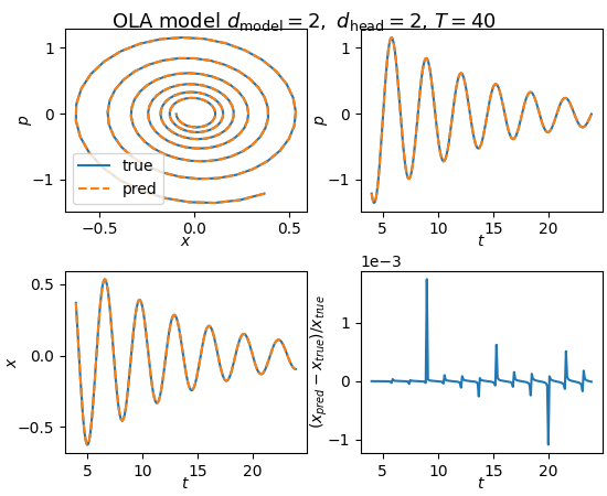
Fig. 1: OLA model training results with $T = 40$ time steps.

Does the model do anything with all the new bandwidth given? This does not seem to be the case. The model here learns to reduce itself to a linear model, eliminating the attention module altogether. This can be first seen by looking at the saliency map. A saliency map in its simplest form tells you how the outputs of the model are changed as you change the inputs. In our notation the output is $\boldsymbol Y_t = (x^{\text{pred}}_{t+1}, p^{\text{pred}}_{t+1})$ and $\boldsymbol X_t = (x_t, p_t)$, and the saliency plot is a map of $\partial Y^\alpha_i / \partial X^\beta_j$ as shown in Fig. 2.

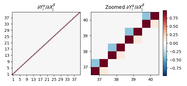
Fig. 2: Saliency map for OLA model with $T = 40$.

The fact that the saliency map is diagonal means that the values of previous tokens do not affect each other. One can further confirm this by looking at the output matrix $W_O$ and in this case we see that it has zeros for all elements. That is, the attention actually writes nothing to the residual stream…

Admittedly this is a whole lot of work for nothing.

Except it is not really for nothing. We learned something. We want to see the attention mechanism in action in the simplest case possible, and our approach here is to start as simple as we can and only make things more complex when we are forced to. We also got familiar with transformers and set the notations.

Making things as complex as they need to be

We need to make the problem harder such that it is no longer linear. I think the simplest, and most interesting way to do this is to allow the natural frequency and damping to vary during training. This forces the model to first learn $\omega_0$ and $\gamma$ from the given input path, then make the prediction for the next time step.

For now, I keep $\gamma$ fixed, and train the model with trajectories having $\omega_0 \in [1.0,4.0]$ and $\gamma = 0.1$. This is how the model performs when given a trajectory with $\omega_0 = 2.0$ at validation

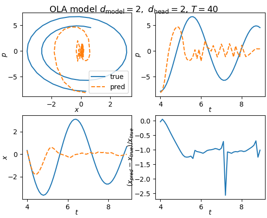
Fig. 3: OLA model cannot learn $\omega_0$ when trained on trajectories with different $\omega_0$.

The model fails to reproduce the dynamics except for a very small number of time steps, and then quickly becomes very wrong. There are many ways we can try to increase the complexity of the model to try to enhance its performance. First thing to try is to increase the dimensions of the residual stream. Here are the results with $d_{\text{model}} = 8$, and $d_{\text{head}} = 4$:

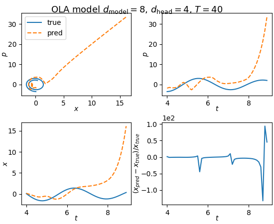
Fig. 4: Changing the residual stream dimensions as well as using 2 attention heads does not seem to help.

This seems to perform worse and does not help.

Next we try moving to a more complicated model. Instead of the one layer attention, we try n-layer attention model (nLA). Here are the results for $n = 8$ with $d_{\text{model}} = 16$, and $d_{\text{head}} = 8$:

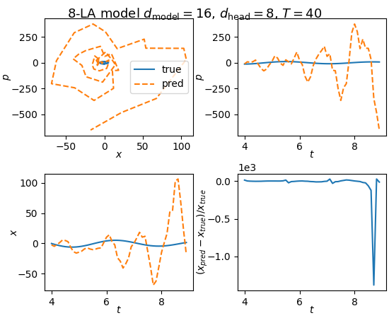
Fig. 5: Adding more attention layers doesn’t seem to help either

This doesn’t seem to do much of anything either.

Interestingly, what seems to help a lot is removing the causal mask in the attention mechanism:

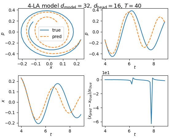
Fig. 6: Removing the causal mask from the attention mechanism seems to help with training and performance quite a bit

I initially added the causal mask because it seemed like a nice physical constraint. However, I don’t see any reason that you must have it. There is no cheating here by removing the causal mask. Increasing the number of layers in the case of no causal attention helps model prediction:

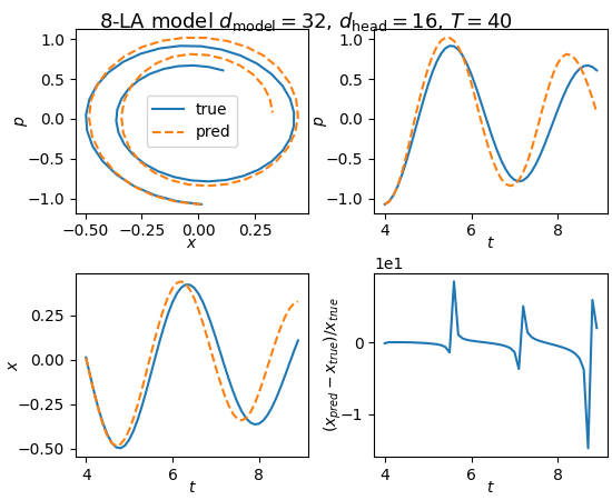
Fig. 7: Adding more layers when we remove causal mask helps performance.

Finally, a quick comparison with linear models. Two things I want to address: 1. How does the performance of the $n$-LA model compare to a simple linear model, and 2. Does the $n$-LA model reduce to a linear model similar to before. I think the following plot addresses both questions:

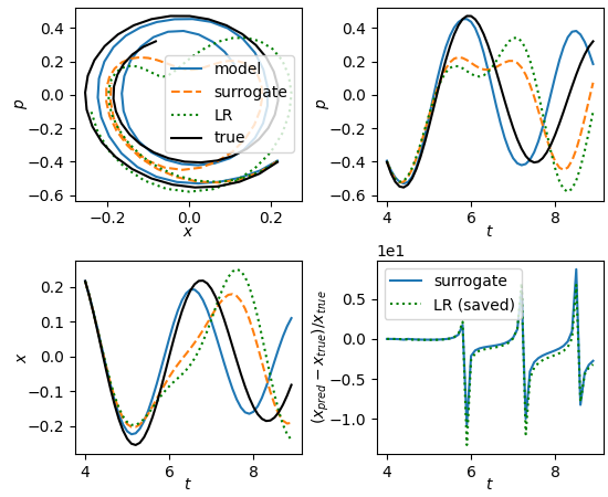
Fig. 8: Comparing $n$-LA model with a linear regression model. Also using a linear model as a surrogate model to see if the $n$-LA model reduces to a linear model.

In the above plot, the model is the $n$-LA model with $n = 8$. At least to my eye, the $n$-LA model seems to track the true trajectory better. Furthermore, we train a surrogate linear model for the $n$-LA model. If the $n$-LA model got reduced to something that is linear then we should be able to train a surrogate model to exactly reproduce its behaviour. This does not seem to be the case, as the trajectory of the surrogate model quickly diverges from that of the original model. I take that as strong evidence that the $n$-LA is not reduced to a linear model.

I’ll have to keep experimenting with the transformer model to improve its accuracy. If you see a reason this task is doomed to fail let me know. If you have ideas about how to make the model better also let me know.